Optimisation in data science: processing billions of GPS coordinates
This post is now many months old. I didn’t publish it at the time because it just got way too long, and to paraphrase Mark Twain, I didn’t have time to make it shorter. The other reservation I had, is that it’s pretty hard to explain why I didn’t (1) use a routing library like Valhalla, or (2) calculate road topology. I speculate about this a little at the end, but in retrospect I think it was mostly a kind of “greedy optimization”: I started with existing code, at each point made a small tweak, and ended up in a local, but not global, optimum.
Still, it may be interesting to some people anyway, so with some free time on my hands, I’ve made a few edits and hit publish.
I spent a part of this week helping some geospatial colleagues process GPS data: without being too specific, they have daily log data for around 1.5 million commercial vehicles in a large country, with each observation spaced a couple of seconds apart. Needless to say, this is a lot of data: around 1TB of data per day.
The project is exploratory, so at this point they were just interested in a “toy” application: traffic counts for Open Street Map ways (roads, roughly). As is pretty typical in the life of a data scientist, they had a prototype analysis running, but there was no way it would scale to the volume of data they had. Initially they came to me to see if I could help them run it on our internal cluster.
Usually when people have speed & scaling issues, my advice is to take their current code and run it on as powerful a machine as possible (faster CPU, more memory and - if their underlying code can take advantage - more cores). This point cannot be retweeted enough:
https://twitter.com/garybernhardt/status/987447046150934528
Hadoop-style clustered computing is pretty ill-suited to the corporate world: it takes specialist skills, which are extremely expensive in most corporate settings, compared with better hardware. Of course, the exact opposite situation prevailed at the likes of Google and Yahoo when these systems were developed.
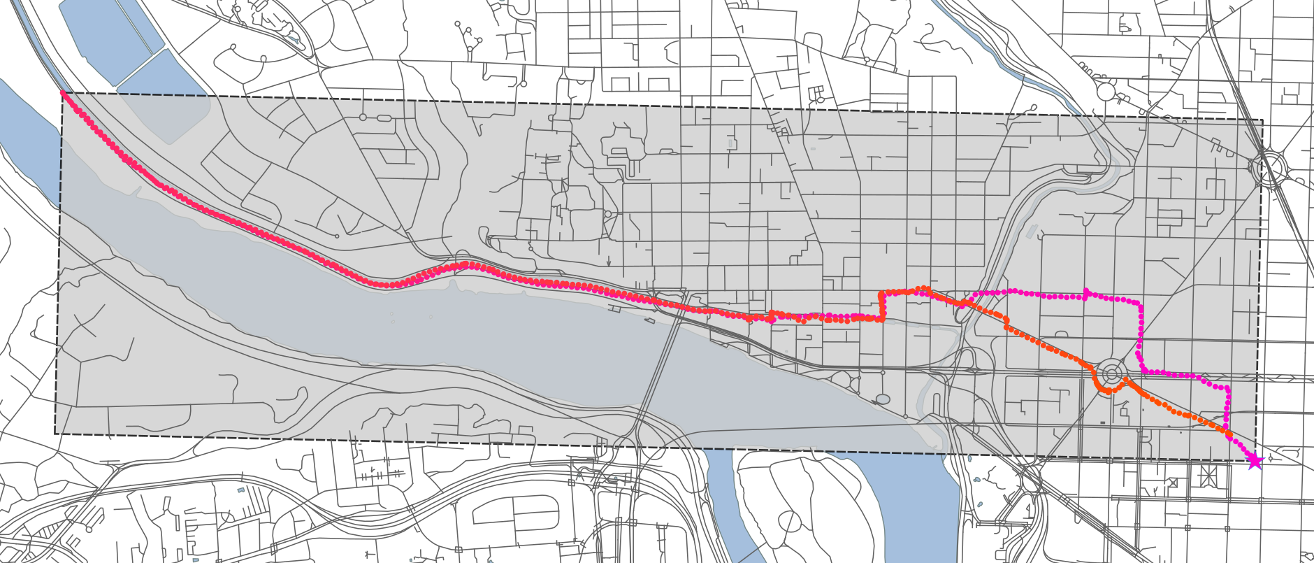
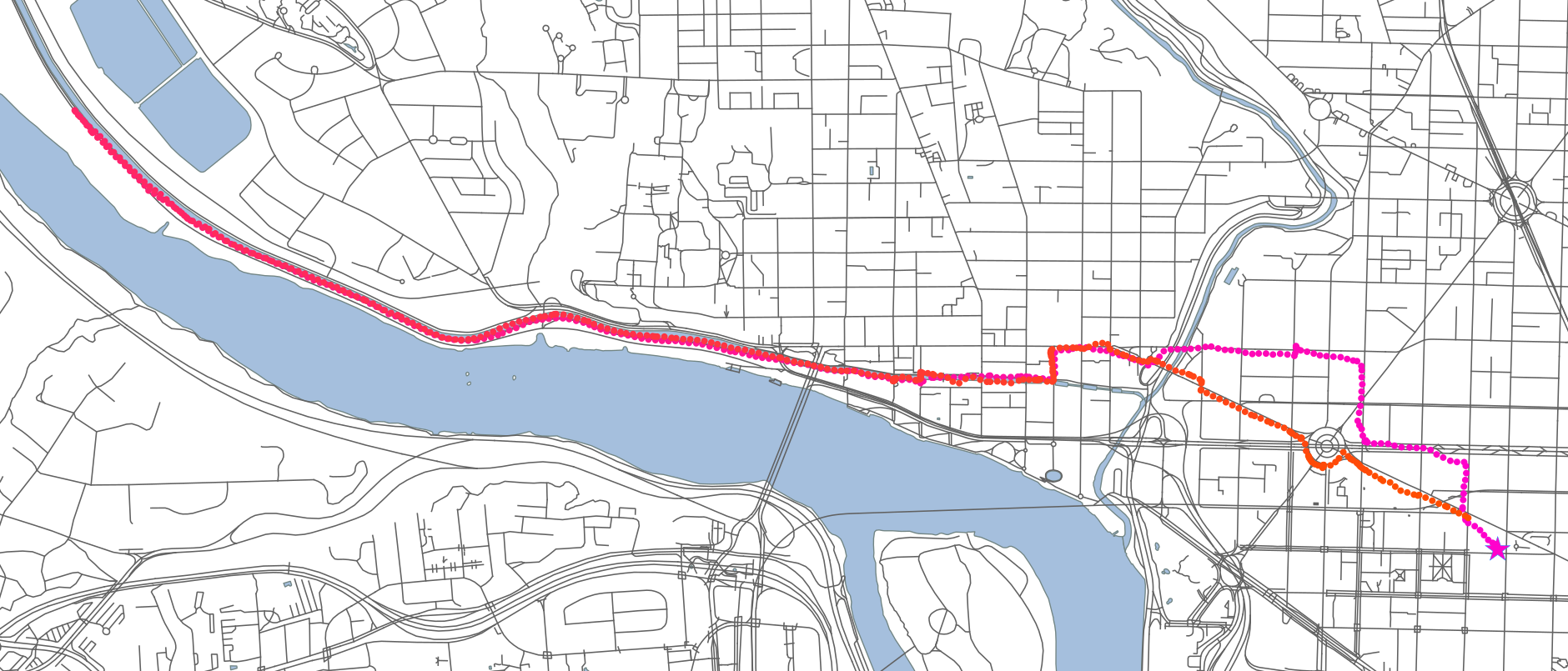
Anyway, in this case it seemed like some optimisation might be helpful before turning to more serious measures. Since I can’t share the data, I’ll use some of my own running data as an example. This is from Thursday night, an 11km run along the C&O canal in Washington DC, starting and ending at the World Bank. Purple is earlier in the run; orange is later; and each dot is around 2 seconds apart.
The proof of concept solution #
The initial concept the team had was really just what you might do interactively in QGIS or ArcGIS as a first cut, then translated into python with geopandas, shapely, etc
First, it splits each vehicle’s day log into 1 hour segments. From that, it calculates a bounding box, and selects only those roads intersecting with the box:
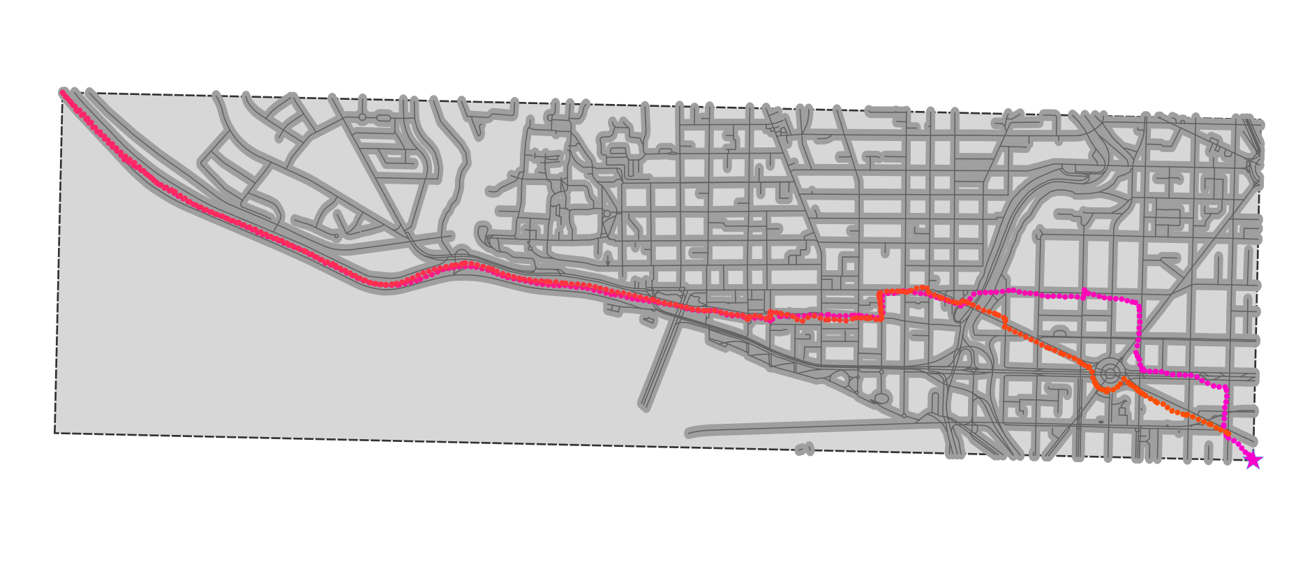
Then, it buffers each road within the selection by a small amount (to allow for the physical width of roads, error in the OSM data, and error in the GPS coordinates):
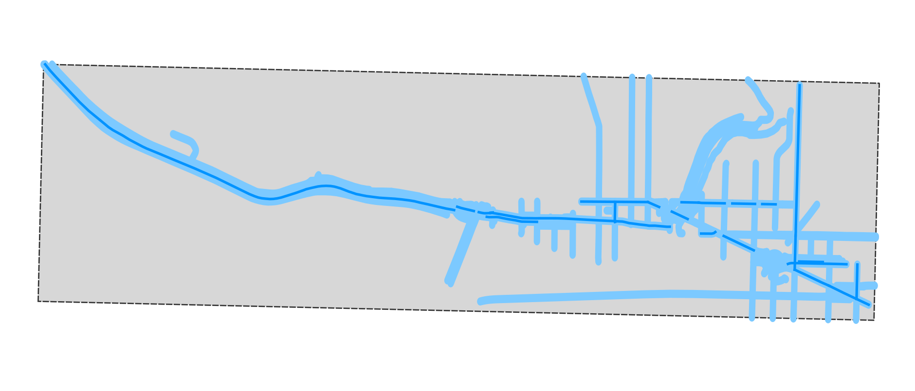
Then, the GPS trace is converted to a connected line, which is intersected with the buffered roads. The result is below:
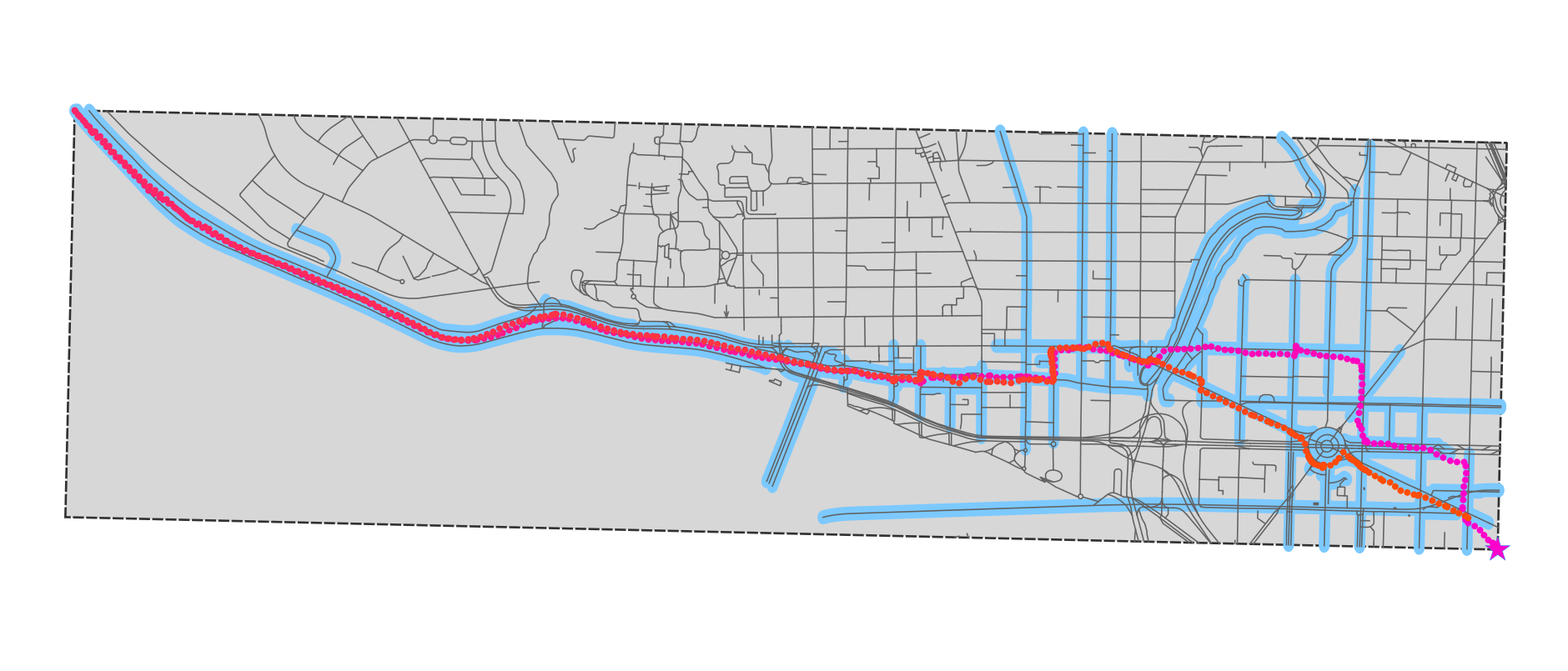
Straight away you can see that this is a pretty rough solution: the buffering means a lot of side streets will spuriously intersect with the GPS trace, even though the vehicle (here: me) never travelled on them.
More immediately, this solution was slow. It took 244 seconds to process a sample of 5 files. Five, out of a total of around 1.5 million per day! Running this code would take around 20,000 hours, or a bit over 2 years, to process a day’s worth of data. Even if we put in the cluster and it ran, say, 500 times faster, that’s still around 40 hours - whereas the data would be accumulating at 24 hours every 24 hours.
Previewing the conclusion, major optimisation of the code, plus single-machine parallelisation, got it down to a much more reasonable runtime of 5-6 hours, processing very close to 1 billion lines (GPS points) per hour. The optimisations were:
| Optimization | Speedup | |
|---|---|---|
| Reframe the problem: requires domain knowledge |
|
15x |
| Improve the algorithm: requires algorithms knowledge |
|
4x |
| Tweak the implementation: requires lower-level platform knowledge |
|
2x |
| Parallelise: requires basic parallel / distributed computing knowledge |
|
5x |
| **TOTAL** | 450x | |
What I think is interesting is that data science requires all these different levels of knowledge (if we consider data science the link between exploratory analysis and production code). In a larger team, on a larger project, these could be divided between multiple people, but I think they’re skills and knowledge that every data scientist should aspire to have.
What follows is a long, blow-by-blow account of the algorithm refinements.
Optimization level 1: reframe the problem (15x) #
This optimization alone delivered the largest benefits: a 15x speedup.
Optimisation often focus on algorithms or code efficiencies, but by far the biggest gains can come with answering a different question. You’re running a regression, but maybe you just need a binary classification. Maybe you don’t need individualised predictions at all.
These kinds of optimisations come from knowing the domain or business area. Unlike more technical optimisations, which should affect the output, they often result in a different solution. Importantly, they usually result from a deeper understanding of the problem, and so often produce a higher quality solution, quite apart from being faster.
I tried a bunch of low effort, technical optimisations - spatial indexing, pre-calculating the buffers, etc - before realising that the solution was fundamentally wrong. As the spurious roads above make obvious, intersection is not the right thing to do here. The set semantics of standard geospatial operations - intersections, unions, differences - make sense for some applications, but not for thinking about journeys, because they throw away something essential to a journey: the arrow of time.
Further, intersection is an expensive operation. And, actually, we don’t really care about intersection. What matters really, is what is the nearest road. Actually, that’s not quite right:
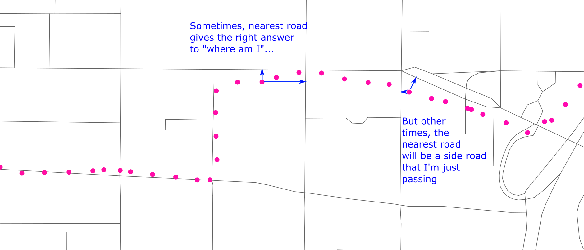
But it’s close. Unfortunately, even figuring out the nearest road would be complicated. The shortest distance won’t generally be to one of the nodes of the way, but to some point part-way along it.
So at this stage, I had an idea for how to reframe the problem, but I wasn’t quite sure how to implement it.
Optimisation 1b: create more data #
This sounds unintuitive, but sometimes the key to speeding up a big data problem is to create even more data (it’s more intuitive if you remember that’s exactly what an index is, whether in a database or a physical library card catalogue).
Many problems involve some sort of join between one not-so-big dataset (size: M), and one big dataset (size: N). This problem is of that sort: the road map is moderate (say ~100MB) but the GPS log data is big (TBs).
Any solution you can imagine is going to look something like this:
- Process the road map - O(M)
- Process the log data - O(N)
- Process both together - O(NM)
Because N is at least 100 time bigger the M here, it makes sense to spend a lot of extra time in the O(M) part, in order to make the O(NM) part as fast as possible. That might include transforming the map data into a form which is faster to use.
My idea was as follows: generate points every 25 metres along each way, to create a discrete, linear mesh of points for each road. And then throw everything into a spatial index (the rtree package, which wraps around libspatialindex).
This appeared to blow up the map data a lot: around 200,000 ways turned into 6+ million points, which is maybe 5-10 times as many as the underlying points that defined those ways.
Here’s that approach, applied to the section of Washington DC where I ran (with points on the same way coloured alike). In the real application, I did this for the entire country in question. This takes around 20 minutes on a single core, but it’s a one-off cost: I save this list of points and just reload it on future runs.
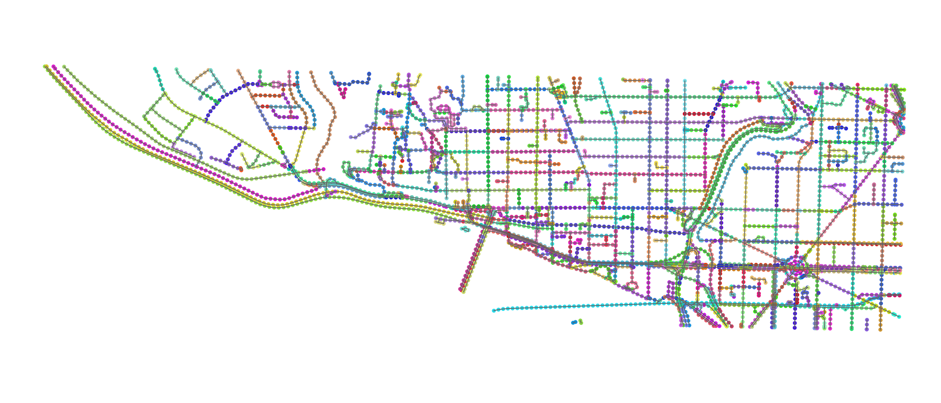
Once the points are generated (or loaded) I feed them all into the RTree, which is a kind of geospatial index that dramatically speeds up queries like “which points are inside the box (x1, y1, x2, y2)?”- from O(M) to O(log M) time.
Now, the algorithm is quite simple. Read in a point from the GPS log. Build a bounding box around it (so, I buffer the vehicle, instead of the road). Look up the road points that are inside the bounding box. If there’s just one, that’s the road I’m on.
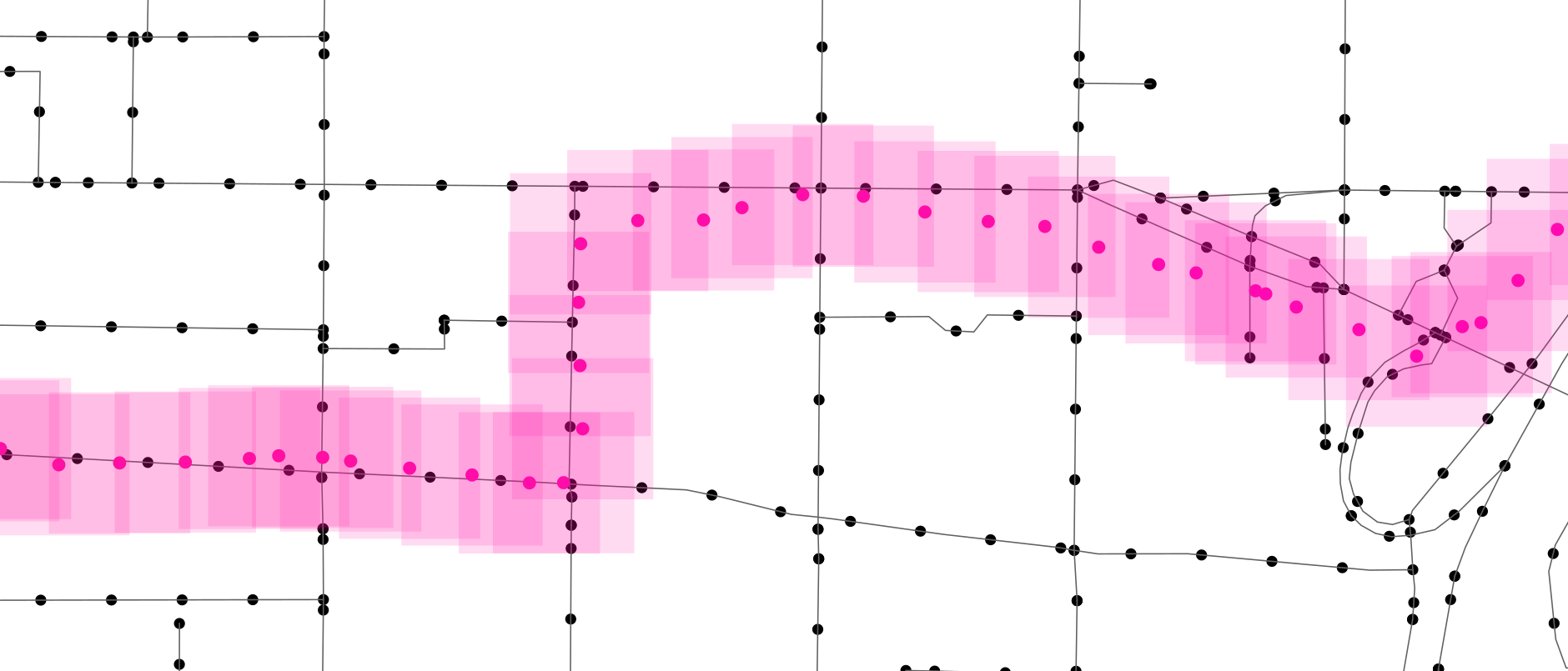
Of course there is a bit more nuance than that, but at this stage the only additional logic I included was this rule: don’t “lock” onto a road until you see at least three points’ travel on that road in consecutive vehicle bounding boxes. Since the road points are equally spaced at 25 metres, this guarantees the vehicle has been travelling on the road for some distance, which rules out spurious side streets.
As I noted above, this delivered a 15x performance benefit, and - almost as a side effect - the result was much better than the intersection based algorithm. You can see that only roads that I actually ran on have been selected (the parts that don’t look that way are just longer OSM ways, which I ran on part of).
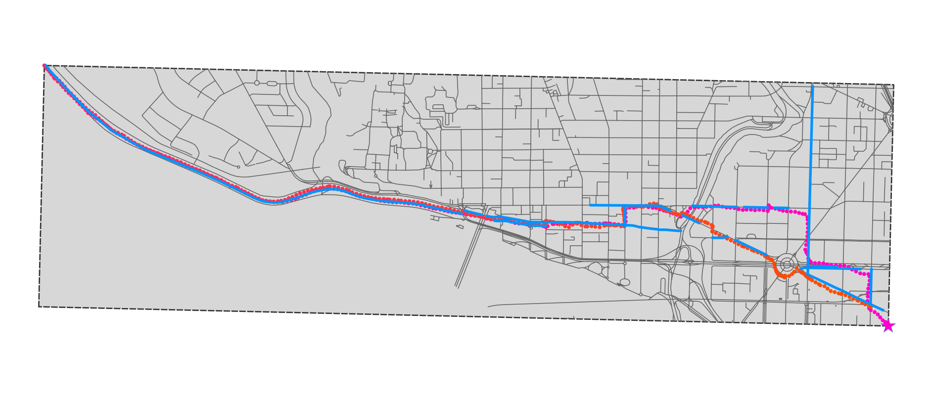
And here’s the comparison, where the thicker blue line is the intersection method and the thinner blue line is the points method. There is one problem, in that the points method will fail to detect very short road segments (e.g. the roundabout at the SE corner), because I wasn’t on it for long enough. But in general it’s much better.
Optimisation level 2: improve the algorithm (4x) #
Next up came some algorithmic improvements: archetypal optimization. The big gains here came from dealing with two special cases.
Lookahead on roads (2x) #
Initially I was looking up every newly read GPS point in the RTree, but this is throwing away information. If a vehicle was previously on a road, it probably still is, so before looking generally in the RTree, it makes sense to see if the new point is in the vicinity of any of the next few markers on the road. This cut out a lot of lookups, and roughly halved the runtime.
Disambiguation #
Initially, if more than one road continued to match the vehicle trace after the required 3 points were seen, the routine didn’t match a road at all. This is a problem since parallel roads are quite a common occurrence, e.g. for high-speed divided highways. Since OpenStreetMap (and the extract I was working with) contains one-way direction information, it was trivial to use this to disambiguate in this case.
This doesn’t solve every ambiguous case: for example the left-hand section of my run is actually on a canal path, which runs parallel to both a bike path and a road, all of which are bidirectional. In a case like this, the routine just chooses arbitrarily (and often, incorrectly - as it did, indeed, on part my run).
It would be possible to do better (using actual distance to the road), but it wouldn’t be straightforward, so we just ignore this issue.
This wasn’t actually intended as an optimization, so much as a quality improvement, but locking onto roads more often does improve the runtime, given the lookahead optimization.
Idling (2x) #
This is a special case I only identified through profiling. After the previous optimizations, I expected the RTree to be consulted only rarely - for, say, less than 1 in 10 GPS points. Instead, profiling showed that it was much higher than that.
It turned out the reason was that these vehicles spend a lot of time basically parked, not on (or very near) a road, and not moving very much (probably stationary + random GPS error), but still transmitting a trace. They’re likely loading and unloading. This was consuming a lot of processing time, because the lack of a road lock meant that every new point caused an RTree lookup.
Instead, I started detecting and tracking this idle state. If a vehicle remained more-or-less stationary inside a box (which is defined dynamically), the routine stops looking for roads - until the vehicle next exits that box. This change eliminated many of the remaining RTree lookups, and halved the runtime.
Optimisation level 3: tweak the implementation (aka ugly hacks) (1.5x) #
So far, most of the optimizations had improved the code - increasing the complexity, definitely, but not in a bad way. The next series of optimizations unquestionable reduced the readability (and even robustness) of the code, and for relatively small benefit - but altogether increased performance by a not-insignificant 1.5x.
When I first profiled the code, the RTree lookups took up about 90% of the runtime, so there wasn’t much point focusing on anything other than (a) reducing the number of those or (b) speeding them up. Option (a) motivated the previous optimizations.
Option (b) seemed more limited, since the RTree is handled inside a compiled C library. But it turns out that there were two small tweaks possible:
-
First, I reduced the size of the objects I stored in the RTree. The rtree package allows you to store arbitrary pickle-able Python objects in the tree, but that doesn’t mean its a good idea, since (a) they take up memory and (b) they will need to be unpickled on each tree lookup, which is relatively slow. So I reduced the indexed object to a minimum, just a two-part id for “which road” / “which point on the road”. The more complex dict objects that I had been storing, I moved to a separate (fast, native python) list of lists. I also used objects=”raw” to further reduce the lookup overhead. (Later when parallelising, the list of lists (of dicts) was itself a problem, taking up 5-6GB. Switching each dict to a tuple reduced that to around 1GB, at a cost to readability.)
-
Later, I eliminated the use of objects entirely, by packing my two-part id into a single 64 bit int, as below. That’s weirdly unpythonic and wouldn’t normally work to speed something up, but it avoids an extra internal call to libspatialindex for each lookup:
def pack_index(roadindex, pointindex):
    return roadindex * (2**32) + pointindex

def unpack_index(int64):
    return divmod(int64, 2**32)
Each of these reduced runtime by around 10 percent.
I added two further optimisations for things that initially represented a small percentage of runtime, but loomed larger as the rest of the code got faster:
- csv.DictReader was now taking up a surprisingly large amount of time, over 10%, so I replaced it with a fast (but fragile) custom reader, which just assumes perfectly-formatted input and produces DictReader compatible output, for another 10% time gain:
def fastreader(f):
  f.readline()
  for line in f:
      fields = line.split(",")
      out = {}
      for c in REDUCED_HEADER_COLS:
          out[HEADERS[c]] = fields[c]
      yield out
- Early on I had converted my colleague’s code from working in WGS84 lon/lat coordinates (ie. degrees of longitude and latitude) to an appropriate UTM zone. This made sense at the time as UTM coordinates are measured in metres, which makes it easy to generate the road markers, size bounding boxes correctly, etc. The problem with this choice was that the GPS trace files were in lon/lat, and converting them (using pyproj) to UTM was taking another ~10% of runtime. So I switched the main processing loop to work in lon/lat (having precalculated the road markers in UTM, and converted them back). The only wrinkle with this was having to adjust latitude distances depending on longitude, not strictly necessary for our country but otherwise a source of error at higher latitudes. But that is a single math.cos(math.radians(lat)) scaling, which is many times faster than whatever pyproj was doing to get correct UTM coordinates.
Optimisation level 4: parallelise (5x) #
In a sense, this is the easy one. Python parallelisation is somewhat complicated by the “global interpreter lock”, which mean that multi-threading only really helps IO-bound tasks. For processor-bound tasks, you have to use the multiprocessing library, which uses OS-level processes instead of threads.
This is frustrating as both the Rtree and list of lists were both large memory-resident structures, and now each process would require a copy. That was another motivation to reduce the size of both.
Ultimately, we ran it on a 6 physical (12 logical) core Windows 10 machine, and got around a 5x speedup, which is pretty typical in my experience. On my dual core Macbook, hyperthreading didn’t seem to help and more subprocesses than physical cores resulted in a slower runtime. By contrast, on the Windows workstation, it offered a slight benefit, taking a similar amount of time with 9, 10, 11 subprocesses (for 6 cores).
Epilogue: the one that got away #
If you’ve read this far, and know something about geospatial data and OpenStreetMap, you’re probably wondering how I missed the most obvious optimization: I don’t take any advantage of the topological / network structure of the roads.
To explain: if road A ends at a four-way junction with roads B, C and D, and the vehicle has just left road A, I shouldn’t need to lookup in the RTree to find the new road - I should really just be able to check B, C and D, because the vehicle is almost certainly on one of those roads now. That would drastically cut the number of expensive RTree lookups, since you would then only have to do those when you re-enter a road having left the road network entirely (e.g. exiting a driveway on private property).
I did think of doing this, but didn’t, for three not-very-good reasons:
-
I thought OpenStreetMap suffered from a large number of unconnected ways. Some quick analysis later showed this is not the case, if it ever was, at least in our country of interest. Moreover this was a weak excuse, since DIY building a network topology from the geospatial data wouldn’t be that hard.
-
I never expected this process to become so elaborate, so I kept avoiding the relatively large fixed design / coding cost of incorporating this information.
-
The original map input my colleague was using was a shapefile, devoid of network topology, and I just accepted this as given. Later, it became something of a game to work with what I was given.
So arguably I missed a pretty fundamental stage in data science, which is to ask** Do I have the best data to answer this question?**
Something for version 2, perhaps!
Add comment
Comments are moderated and will not appear immediately.